How Python Lists Work Under the Hood with a Baseball Example

If you have programmed in Python in any capacity, then you are most likely familiar with the python list. It is one of the most popular built-in data structures in python and has many applications.

Characteristics of the Python List

The list is a sequential data type because it is indexed. The list is zero-indexed meaning that the first element in a list is referred to as 0, the second element as one, the third as two and so on.

x = [9, 3, 1, 12, 18]
x[0]
Output: 9

The python list differs from similar array data types in other programming languages because it can contain elements of any type. This allows for great flexibility to the programmer including the ability to store other abstract data types within the list including lists themselves.

x = [3.1415, 'Hello World', ['test', 7.8, 13]]
x
Output: [3.1415, 'Hello World', ['test', 7.8, 13]]

Lastly, the python list is mutable. This means that the any element in the list can be changed or deleted and the list can be appended too. Lists being mutable provides another form of flexibility.

x[0] = 3
x[1] = 'Cuse'
x
Output: [3, 'Cuse', ['test', 7.8, 13]]

Array Implementation

If some of the characteristics of a python list seemed obvious or was a review, that’s fine. However, it is important to know how the list compares to similar data structures in other programming languages.

Earlier, I compared the list to an array. The list is python’s implementation of the array data structure. If you are to take a CS course on data structures, you will certainly learn about arrays – a collection of elements that are identified by their index. The list follows these basic characteristics and implements their own as mentioned above.

The array data structure can further be broken down into two categories:

1. Static Array: The maximum number of elements in the array are established and cannot be exceeded.
2. Dynamic Array: There is an arbitrary maximum number of elements allowed in the array and if exceeded, the array will grow to some new maximum number of elements to accommodate the new element and anticipate future elements. The python list is implemented specifically as a dynamic array. I will include a nice example later to help you understand the definition above.

Big-O Notation

Before I implement an example, I want to explain the Big-O Notation because it’s important to understand the time complexity of certain operations on the list. This will help you know in what situations that a list is the best data structure to use.

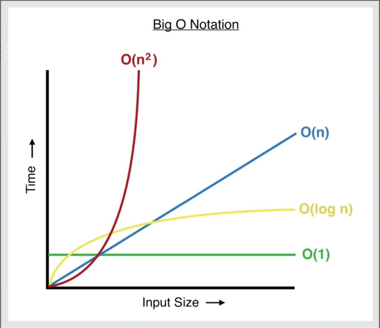
As seen above, Big-O is represented as a function in terms of n to a certain power. N represents the number of elements the algorithm is operating on and you imagine the growth of the function as n approaches infinity. This helps you understand the time complexity of functions for very large values of n.

We prefer an operation or algorithm with a time complexity of O(n) over O(n2) because for very large values of n, the time complexity (represented by the y-axis on the graph) is substantially better.

Baseball Example

Imagine you play on a baseball team and you want to store the number of hits you have each game. Because the games occur sequentially you can store the number of hits for each game in a list. After four games you have: 3 hits in the first game, 2 in the second, 0 in the third and 4 for in the fourth.

You can create a list to store this data:

hits = [3, 2, 0, 4]

If we were able to see how the hits list is stored in memory, it would appear something like this:

Early I mentioned how the list is implemented as a dynamic array. We will pretend that python assigns the list a max size of 4 elements. The dark gray boxes symbolize other areas of memory being used by different programs. The memory representation on the left is a simplification because ints in python require 32 bytes of memory and since each register is 1 byte, an int is stored in 4 contiguous registers.

Accessing an item in the list

If you want to know how many hits you had in a certain game you would use the game number minus one as the index. For instance, to lookup the number of hits in the third game:

hits[2]
Output: 0

Accessing the element in memory would look like:

Accessing an element by its index is as simple as taking the location of the root index and adding the search index times the size of each integer which in this case is four bytes. Because accessing by index requires one computation, it has a time complexity of O(1).

Adding an element to a list

You then play the fifth game of the season where you mash five base hits. You update your hits list by doing:

hits.append(5)
hits 
Output: [3, 2, 0, 4, 5]

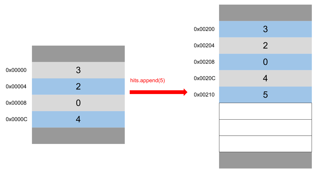
Now on the surface level its seems that appending an item to the list would have a constant time complexity of O(1). However, if we take a look at the the list in memory, that isn’t necessarily the case:

Because the original list had a maximum capacity of four elements, adding the fifth element in this case required for the list to be relocated in memory. The list now has a maximum capacity of eight elements. This is what I meant when I said that dynamic arrays grows to append the new element and anticipate future elements.

So in this scenario appending an element had a time complexity of O(n) because it had to move n elements. However, this is the worse case scenario and because python’s algorithm for the dynamic array is so efficient, appending items has an average time complexity of O(1).

Deleting an item from a list

Since in your second game you only completed five innings due to a rainout instead of the minimum of six innings, your hits do not count for that game. To delete the number of hits for the second game you would do:

del hits[1]
hits
Outcome: [3, 0, 4, 5]

If you look under the hood at the memory:

When deleting an element from a list, every element after the specified index is shifted upwards by one index in memory. The closer the deleted element is to the root index, the more elements that must be shifted. Therefore, the worse case time complexity of deleting an element in O(n) because if you delete the root element, n elements in memory are shifted.

Inserting an item in a list

You forgot to include the number of hits for what was officially your third game so you do:

hits.insert(2, 1)
hits
Output: [3, 0, 1, 4, 5]

Inserting 1 hit for the third game causes a shift in memory:

When inserting an element in a list, the element at the specified index and the elements after must be shifted by one index in memory to incorporate the new element. Again, operations towards the front of the list cause more elements to be shifted resulting in a worse case time complexity of O(n).

Iterating through a list

You forgot what game you had 4 hits in so you iterate through each game and stop at the index where the number of hits equals 4:

for i in range(len(hits)):
    if hits[i] == 4:
        break
i + 1
Output: 4

If the game you had four hits in turned out to be the last game, then you would have had to look through the entire hits list. Therefore, the worst case time complexity is O(n).

Summary

To recap, a list in python is implemented as a dynamic array that grows as more elements are added. A list is indexed, can contain multiple data types, and is mutable.

Since accessing an element by index has a time complexity of O(1) and the average case time complexity of appending an element is O(1) , the list is a good data structure for handling sequential data streams.

Lists struggle however when handling insertion and deletion due to its O(n) time complexity. This is where other sequential data types like the linked list fare better.